Trying to Win Last Man Standing with Statistics

Every year my old hockey club Preston run a game called Last Man Standing. The basic premise is to pick a team each week, if they win, you stay in, otherwise you are out. It costs £10 to enter, with £5 going to the prize pot, and £5 going as a generous donation to the club. I want to win - and not by blind luck (like Matt Cav did a few years ago).

Although the club are very generous and allow you to have theoretically as many entries as you like, there is a number of entries you could have that could almost guarantee a win. At the start of my PhD, my supervisor got me to learn this course, where one example used information theory to find the number of tickets you would need to buy to guarantee winning a lottery. I imagine a similar approach exists to this (and would be quite a nice quant interview question)- but nobody likes the guy who brute forces everything. I instead entered 3 times, because “Anything can happen in football when you don’t take care of key moments.” – Liam Rosenior.

So: the plan. First, need to find match outcome probabilities for each fixture. Then, when I have these probabilities, find the “optimal” team choices to maximise my chances of winning (spoiler: I didn’t spend very long on this so is less exciting)…

Finding Match Probabilities

The first part of the plan was to find the probability of a win draw or loss for each fixture every week. We could easily use a proxy, like the average of all bookmakers odds (i.e. if we have odds 5/4, then the “implied probability is 4/(4+5) = 4/9 = 44.44%). However, there are 3 main issues with this:

• Implied probabilities won’t always sum to 1 as the bookmakers price odds in order to always make money
• Bet flow will alter odds - if true probability of Lucas Paqueta getting a yellow card is 1%, then all of Paqueta island bet on him getting one, to hedge their exposure the bookmaker shifts their odds and increases the implied probability (note this is just a random made up example and has no connection to real life)
• I don’t get to do any calculations myself

Hierarchical Approach

To find a probability of a match outcome, I decided to utilise Monte-Carlo simulations. The idea is to build a statistical model for an event happening, sample a realisation of this model, and then simulate the process. We do this in two steps.

My idea is to build a model for a given teams shot count for and against (for home and away, due to the statistically significant home advantage). Then, build a second model around the teams xG distribution, which models goal probability for a given shot (extensive discussion here).

Then, to simulate a match; we sample the number of shots a team might have. One realisation might be that Everton have 10 shots against Bournemouth. Then for each of the 10 shots, we draw a realisation from the xG distribution, and a random number. If the drawn value is higher than the random number, we assign +1 goal for Everton, else stays the same. We then simulate the same match a large number of times (~10,000 times), to play the game ~10,000 times, to find 10,000 different numbers of shots Everton have, and the number of those shots that result in a goal. Each of these 10,000 simulations produces an outcome (i.e. Everton win, draw or Bournemouth win), and then the number of occurrences gives an estimate for the outcome probabilities.

Modelling Shot Counts

Shots are discrete count data, meaning there are generally two distributions we could use the model the output; Negative Binomial and Poisson Distributions. Negative Binomial measures the number of failures for a sequence of Bernoulli trials with a fixed probability. Poisson distributions model “rare events” data occurring in a fixed period of time. Generally, Negative Binomial is used when variance is larger than the mean, whereas the Poisson distribution has equal variance and mean.

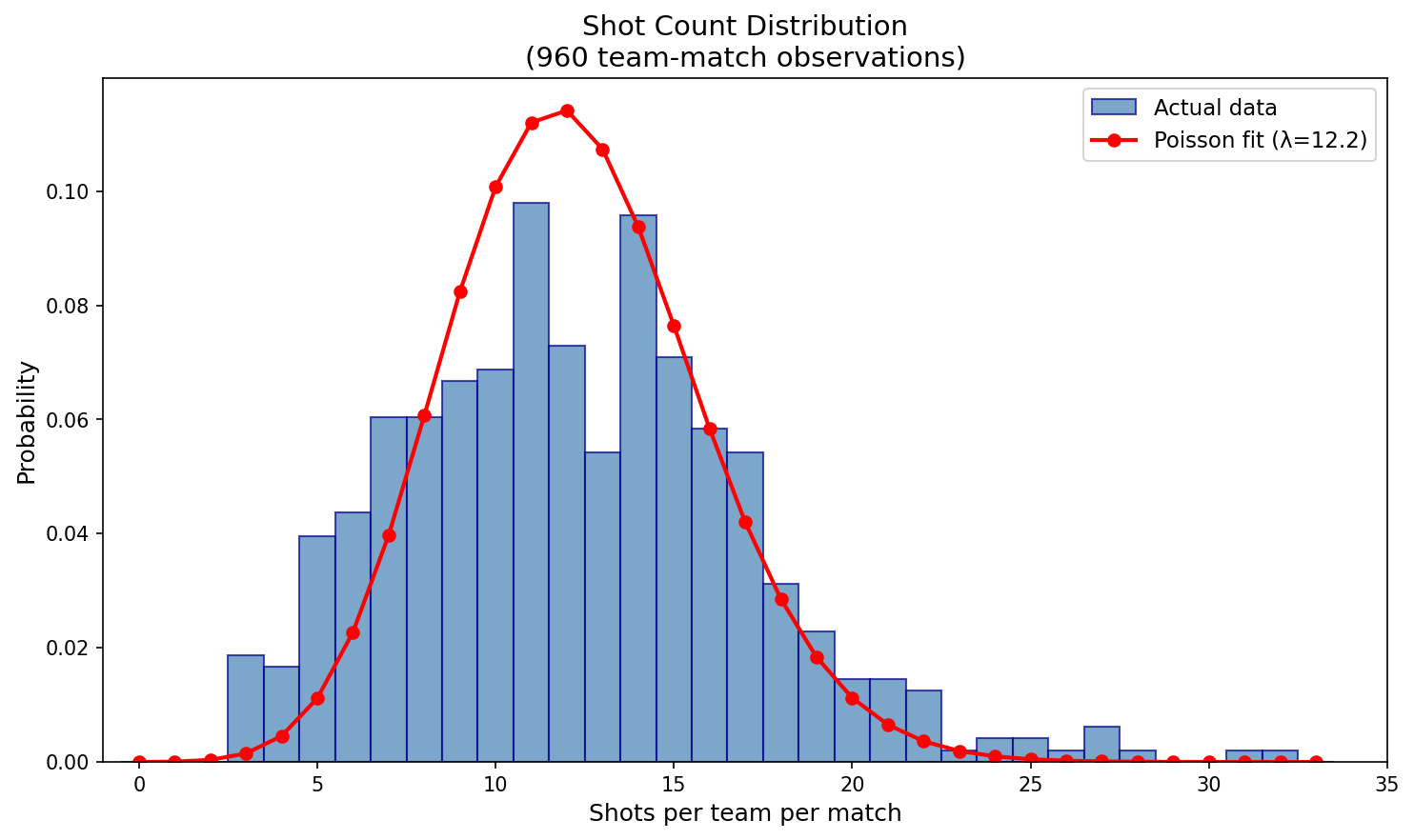
I decided to use the Poisson distribution to model each teams shots, with the parameter $\lambda$.

A conjugate prior is one such that when combined with a given likelihood, the posterior is then of the same form as the prior. This is another reason to choose a Poisson likelihood - the conjugate prior is a Gamma distribution. This is defined over the positive real numbers. As a result, we can take a Bayesian approach to estimating a teams given shots.

\[p(\lambda) \sim \operatorname{Gamma}(\alpha, \beta)\]

Where $\lambda$ is our parameter in the Poisson model, $\alpha$ is a shape parameter, and $\beta$ is a rate parameter. We can take these as hyperpriors, and just use these values as the average over all the leagues.

Combined with each team’s shot data, we can infer a posterior, which allows us to predict future shots for each team:

\begin{align} p(\lambda \mid D) & \propto \prod \frac{\lambda^{x_i} \exp(- \lambda)}{x_i!}\times \frac{\beta^\alpha}{\Gamma(\alpha)} \lambda^{\alpha -1} \exp (-\beta \lambda) \newline & \propto \lambda^{\sum x_i + \alpha - 1} \exp((n+\beta)\lambda) \end{align}

This posterior on the Poisson parameter is then Gamma distributed. For a new match, we are able to sample the rate parameter from this posterior, $\lambda \sim \operatorname{Gamma}(\hat{\alpha}, \hat{\beta})$, then put this into our Poisson distribution to sample a shot number for a given team. For each of these shots, we can then sample an xG distribution, and use Monte-Carlo simulations to get an outcome of the match.

Now, onto xG modelling…

Modelling xG Distributions

xG tends to follow a more complex, empirical distribution that assigns a probability of a goal depending on factors such as shot location, type of shot (header, weak foot etc.) which varies depending on particular model. Generally, these are multimodal, and vary for each team; i.e. Man City tend to generate more high quality chances than Wolves for example.

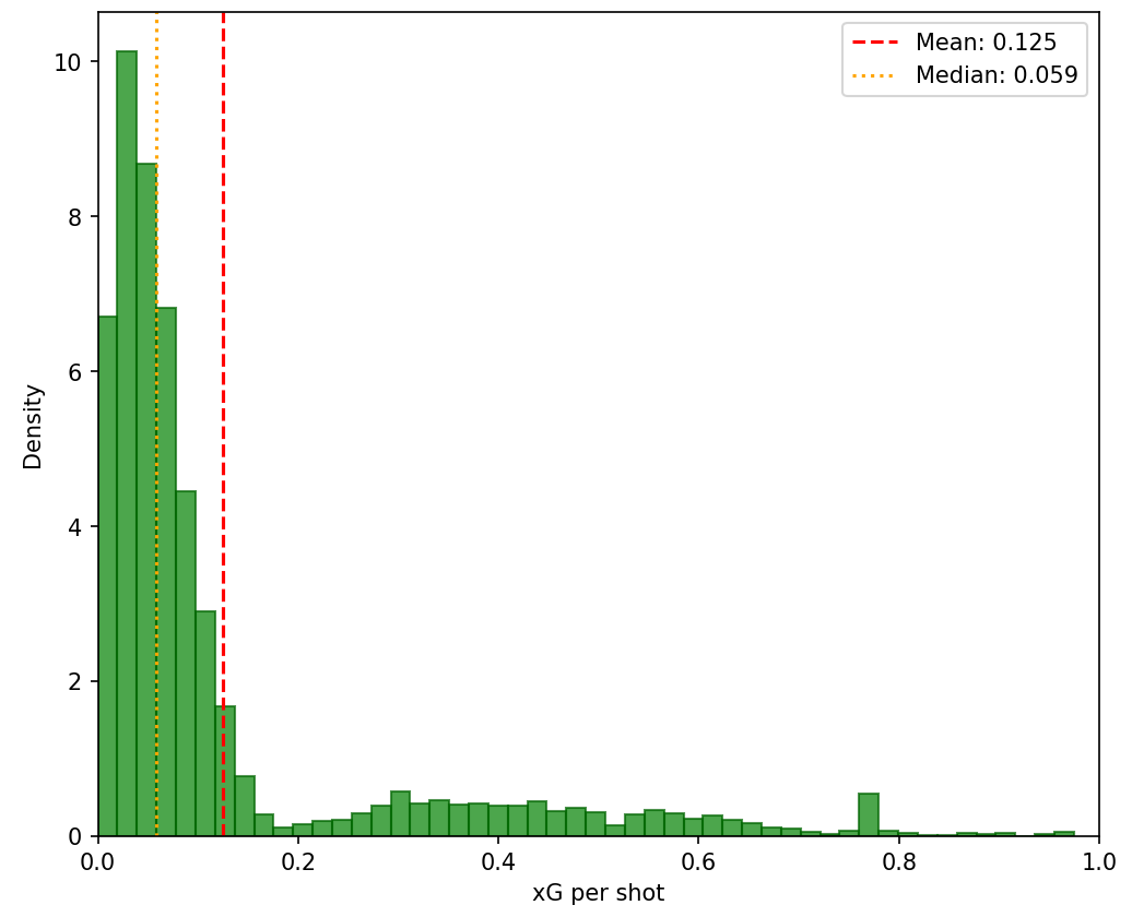
We want to find a posterior distribution for a teams xG - which is the goal probability. This number is on the interval $[0, 1]$, and from looking at the above figure, this looks like it is multimodal. As such we can exploit a mixture of Beta distributions. Beta distributions, $\operatorname{Beta}(a,b)$ have support over the desired interval. Mixtures of this allow us to express the more complex nature of the xG distribution. This time, we exploit an algorithm known as Exploitation Maximisation (EM), rather than conjugate likelihoods. Mixture of Beta distributions have the following density:

\begin{align} p(x) &= \sum_{k=1}^{K} \pi_k \, \operatorname{Beta}(x \mid a_k, b_k), \end{align}

Essentially, we treat the model weights as a latent random variable, and place a Dirichlet prior over them.

\begin{align} & z \sim \text{Categorical}(\pi_1, \dots, \pi_K), \newline & x \mid z = k \sim \operatorname{Beta}(a_k, b_k). \newline & (\pi_1, \dots, \pi_K) \sim \operatorname{Dirichlet}(\alpha_1, \dots, \alpha_K). \end{align}

EM alternates between assigning each xG value probabilistically to a component and updating the Beta parameters to best fit those assignments.

Simulating Future Gameweeks

For each fixture, we construct separate home and away attacking and defensive distributions using historical for and against data. We first sample a Gamma distribution to model the Poisson rate, and then build a Beta distribution to represent shot conversion probability (xG).

For each game we can draw a number of shots, and then iterate through each shot and draw an xG value from our Beta mixture. Using Monte-Carlo methods, we then decide whether the simulated shot is a goal or not. We can repeat this thousands of times, and this should then give implicit win probabilities.

Picking Our Teams Each Week

Unfortunately, this part is less glamorous mathematically — but still quite important. Once we have win probabilities for every team in every future fixture, the problem becomes:

How do we pick teams each week to maximise our overall chance of surviving?

If we let $p_{i,t}$ denote the probability that team $i$ wins in week $t$. If we pick teams $i_1, i_2, \dots, i_T$, our total survival probability is

\[\prod_{t=1}^{T} p_{i_t,t}.\]

In practise we maxmise the logarithm of this.

\[\sum_{t=1}^{T} \log p_{i_t,t}.\]

A naive greedy strategy might just pick the highest probability team each week, but obviously once you’ve picked a team, you can’t pick them again - this might not be advantageous i.e. if Man City have a 70\% chance this week but 85\% next week. To account for this, we introduce a “discount factor”:

\[V_{i,t} = \log(p_{i,t}) + \gamma \, F_{i,t},\]

where $F_{i,t}$ is the average future win probability for team $i$, and $\gamma$ controls how much we care about the future versus the current week.

In words:

• $\log(p_{i,t})$ rewards strong picks now
• $F_{i,t}$ rewards teams with good future fixtures
• $\gamma$ balances greed vs patience

Each week, I rank all available teams by $V_{i,t}$ and assign them to my entries, subject to:

• No entry can reuse a team
• Any entry can’t pick the same team
• Any entry can’t pick opposite sides of the same match

As I had little time, rather than solving this as an optimisation problem, I use a greedy assignment: go down the ranked list and allocate the best available valid team to each entry Although this is definitely not optimal, it probably gives me a better chance than usual, and I had fun doing it.

The overall choices were then:

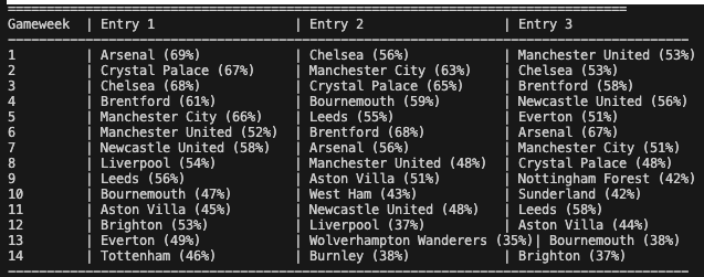
Update as of 27th Feb: were down to 2 entries, as Chelsea and Palace let me down in entries 1 and 3…

Final Update We did not win. It could be interesting to see how many teams we would have to pick to brute force it however. There’s always next year.